Workforce
Preliminary Wages
JobsEQ now includes preliminary estimates for occupation wages in order to provide timely compensation data. These data build upon the BLS OEWS data...
A good estimate of occupation employment at the local geographic level is a critical piece of labor data. How is such an estimate made in JobsEQ, and...
A good estimate of occupation employment at the local geographic level is a critical piece of labor data. How is such an estimate made in JobsEQ, and what are the advantages of using these data in comparison to retrieving an occupation estimate straight from the Bureau of Labor Statistics (BLS)?
The BLS provides local occupation employment estimates through the OES program (Occupation Employment Statistics) for metropolitan and nonmetropolitan areas. These data are an outstanding resource; indeed, they are the standard to which any other estimates should be compared. Nevertheless, there are several issues that users of these data need to be aware of.
First, the OES data are not disclosed for all occupations. In the May 2016 Knoxville metro area data, for example, over a third of the detailed-level occupations (6-digit SOC codes) have no employment information available. So, while most occupations—especially the larger ones—have estimates provided, you cannot find employment counts in Knoxville for occupations such as Pharmacy Aides, Materials Engineers, and Electronic Equipment Assemblers.
Next, the data can be a bit outdated. The May 2016 estimates were released in March 2017. These 2016 data will continue to be the latest available until around March 2018. The occupation data will thus range from ten to twenty-one months out-of-date. While this may not be a big issue in some regions, the occupation employment will likely change substantially if there is significant job growth, contractions, or shifts in the mix of industries.
Additionally, OES data do not cover all types of employment. The self-employed are excluded as well as private households and most of agriculture. By missing the self-employed piece alone, estimates for many occupations are significantly understated. For example, Dentists and Lawyers will be short--on average--by about 20%; Carpenters and Food Service Managers could be understated by more than 30%; and over half of the Exercise Physiologists and Real Estate Sales Agents will likely be unaccounted for.
Further, the OES data are not available for geographies smaller than metropolitan and nonmetropolitan regions. If you need estimates for a single county or a commuting distance from a zip code, the metropolitan or nonmetropolitan data may not be nearly specific enough.
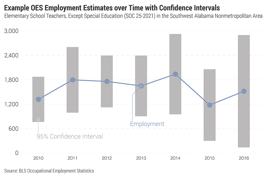
Finally, while the OES data are gathered via surveys of regional employers—indisputably a great primary resource—the sample sizes may not be large enough to get precise and firm results. For example, the Southwest Alabama Nonmetropolitan Area is a collection of twelve counties near the metro of Mobile. This region’s OES estimate of employment for Elementary School Teachers (SOC 25-2021)—an occupation with typically little job variance year to year—bounced from 1,650 in 2013 to 1,940 in 2014 to 1,180 in 2015. The industry employment available for Elementary and Secondary Schools (NAICS 6111) in this region doesn’t indicate any unusual events that would cause such extreme swings in employment to actually occur.
One reason for erratic estimates is that, when working with a small sample size, survey-driven results can veer off from time to time. Indeed, the BLS is transparent about disclosing the uncertainty of these estimates. For example, the value of 1,940 teachers in Southwest Alabama in 2014 was accompanied by a published Relative Standard Error of 26%. In other words, this particular employment estimate would have a 95% confidence interval of about ± 1,000 jobs.[1]
Now, the above[2] was just one example cherry-picked from the data. While there are certainly others like it, a greater amount are likely to be more stable over time with tighter windows of uncertainty.[3] Nevertheless, even just a few examples of imprecise data raise the issue of needing a way to produce more consistently reliable estimates.
Regional planners need both good and stable estimates of local occupation employment. As detailed above, the OES estimates may not fit this need for a variety of reasons. The occupation employment estimates in JobsEQ try to address these issues while still using the OES information as a guide and standard.
One piece of this approach is leveraging industry staffing patterns.[4] Using the staffing mix of industries to estimate employment allows for use of the very latest industry data, which builds on the highly regarded QCEW data set,[5] and which in JobsEQ is typically only three to five months behind the present date. Furthermore, this approach allows JobsEQ to make estimates at the county or zip code level. And, finally, it allows for estimates of all occupations, circumventing the non-disclosure problem.
That being said, the regional OES estimates are not simply ignored. JobsEQ does incorporate these data, but only to the extent indicated by the confidence intervals. That way, variations due to year-to-year sampling changes will not cause erratic changes in employment estimates. Moreover, JobsEQ uses the OES state-level estimates rather than metro and non-metro estimates as the state estimates allow for local variation while also being generally more complete, stable, and built upon larger sample sizes.
In addition to everything mentioned above, JobsEQ also brings in regional estimates for the industries missing from OES (agriculture, etc.), as well as the mix of regional self-employed occupations. As it is important for these additional estimates to be grounded in solid source data, JobsEQ creates estimates consistent with the data available in another BLS data set--the Employment Projections program.
Overall, JobsEQ’s approach allows occupation employment estimates to be consistent with the published OES data while also avoiding the associated problems of relying only upon that source.
If you are interested in a demo of the JobsEQ system, or simply want to learn more about the data, please contact us and we’d be more than happy to speak with you.
[1] To be precise, the 95% confidence interval is ±1.96*RSE, which is 989 jobs. Thus, in this case, the BLS is indicating that--accounting for the uncertainty from sampling errors--it can say with 95% confidence that the actual employment of teachers falls somewhere between 951 and 2,929.
[2] While the BLS cautions, “The Bureau of Labor Statistics at present does not use or encourage the use of OES data for time-series analysis…,” note that with this graphic we are not performing a traditional time-series analysis, looking at the year-to-year change for the purpose of trying to measure the change over time, but rather we are considering the data sequentially for the purpose of examining the reliability of these point-in-time estimates.
[3] Furthermore, this isn’t the only example of uncertainty and changes in these data. The categorization of occupations has inherent uncertainty. Many occupations are similar to one another and classifying a job into one occupation versus another can be subjective. Indeed, the entire categorization system is constantly changing—the current 2010 system will be soon giving way to the 2018 SOC revision which is currently in process. In can be expected with this update that some codes will be added, others deleted, and the definitions of still others revised.
[4] The origin of complete set of staffing patterns really deserves a discussion unto itself—which is beyond the scope of this piece. Suffice it to say, the BLS is again a great resource in laying out most of these staffing patterns.
[5] The Quarterly Census of Employment and Wages (QCEW) is derived from quarterly reports filed by almost every employer in the nation. This data set has issues as well—non-disclosures, timeliness, and lack of published sub-county level estimates—but how those points are addressed in JobsEQ data requires a separate article.
JobsEQ now includes preliminary estimates for occupation wages in order to provide timely compensation data. These data build upon the BLS OEWS data...
Preliminary Estimates is an often-overlooked feature of JobsEQ . What these data are and why they are valuable is described below. The...
“High-skill job groups are projected to continue pacing occupational growth as groups requiring the most education and training are estimated to...